The code was developed and tested on an Intel Pentium 330MHz with 128MB main memory, 512KB cache and Linux operating system (Kernel 2.0.35). The compiler used on this platform was the g77 GNU Fortran compiler version 0.5.19.1. The only optimizing compiler options which have been used are -fthread-jumps and -fdefer-pop. Care was taken that no similar computationally intensive process was running during the time the case study was benchmarked.
Additional tests have been made on a
Silicon Graphics Challenge-L with 8 CPUs (200MHz, 4MB secondary cache
each), equipped with IRIX 5.3 operating system and
SGI MIPSpro f77 compiler, and on a Silicon Graphics Indigo![]() with IP26 board and IRIX64 6.1 operating system. On these platforms, only
the -static compiler option has been used. No porting problems have
been experienced. Tests made using shorter time periods confirmed that all
machines produced the same numerical values up to 5-6 digits of accuracy.
with IP26 board and IRIX64 6.1 operating system. On these platforms, only
the -static compiler option has been used. No porting problems have
been experienced. Tests made using shorter time periods confirmed that all
machines produced the same numerical values up to 5-6 digits of accuracy.
The code compiled also on a Sun UltraSparc with f77 compiler version 4.0. However, the resulting code was not able to handle the requested number of input files.
On all platforms, computation times have been obtained with the UNIX time command.
Preparing the input files by some filter and interpolation routines took 13 minutes on the Intel platform. After that, the MESOPAC preprocessor needed 30 minutes user time on the Intel, 69 minutes user time on the SGI Challenge, and 116 minutes on the Indigo to process the data described above. As a consequence, all further optimization runs on the SGI platforms have been postponed. The resulting data file containing the wind field and other meteorological variables had a size of ca. 250MB. Moreover, the meteorological input data files need an additional amount of disk space of ca. 12MB. Consequently, it has to be expected that a full year simulation takes about 4 hours time on the Intel platform and consumes ca. 1.9GB disk space.
OLAF saves all the time-dependent pollutant masses in the different compartments into temporary files. For the case study considered here, each temporary file needs ca. 25MB of disk space. Given that 10 compartments are used and the meteorological dispersion code writes some additional files, the amount of disk space needed by OLAF for this case study sums up to ca. 325MB (not counting the preprocessor files). Note that after the end of the optimization run these files stay on disk to allow for further investigation of the computed parameters.
Figure Figure 6.10 shows some approximated level curves of
the effect function ![]() for the starting
point
for the starting
point ![]() , while Figure 6.11
(p.
, while Figure 6.11
(p. ![]() ) shows the effect function
) shows the effect function ![]() overlayed over a map of the region considered.
overlayed over a map of the region considered.
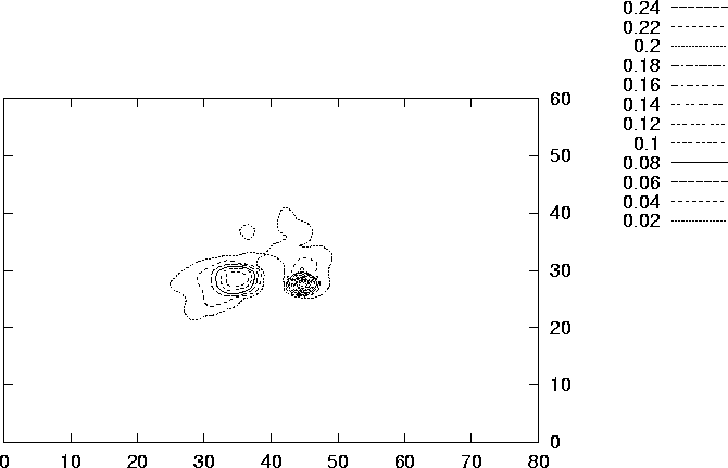
Figure 6.10: Some approximated level curves of the effect function
![]() for the starting configuration.
for the starting configuration.
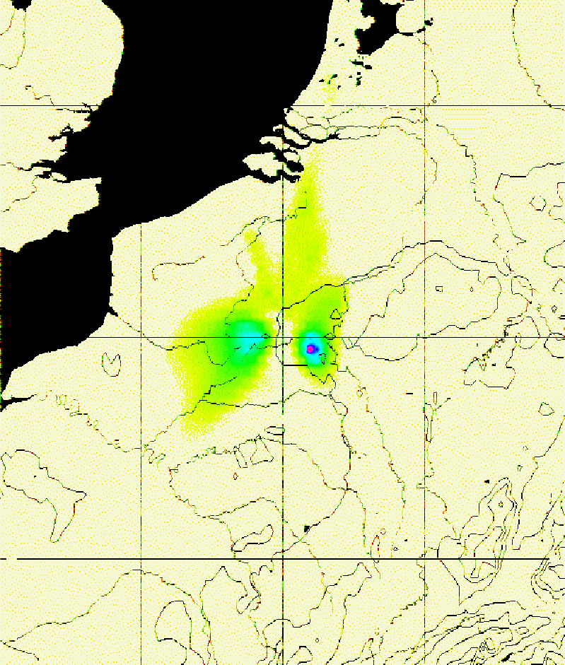
Figure 6.11: The effect function ![]() for the starting
configuration.
for the starting
configuration.
Starting from an objective function value of 70.193, the code needed
ca. 260 hours to calculate a local minimum with objective function value
of 29.018. The final point is

To reach this point, the code needed 23 iterations and 201 function evaluations.
While this number seems to be comparatively large, one has to take into
account the fact that two of the derivatives are approximated by central
differences. Therefore, each gradient evaluation (of which there is one
per iteration step) needs 4 function evaluations. All other function evaluations
are made during the simple Armijo-type linesearch. Therefore, it has to be
expected that more efficient line search mechanisms can decrease the number
of function evaluations significantly. Note that the stack height and width
remain virtually unchanged. This might indicate that the pollution load
is insensitive to small scale changes of these variables on the data used.
Alternatively, one might have a scaling problem here, and a rescaling of
the variables might be in order.
It has to be noted that the relative decrease of the objective function value,
![]() , cannot serve as a measure for the efficency
of the code. In fact, Figure 6.3 shows that the function
value of the starting point can be made rather large simply by placing
the polluting facility as close to Paris as possible. Therefore, the quotient
above has to meaningful interpretation.
, cannot serve as a measure for the efficency
of the code. In fact, Figure 6.3 shows that the function
value of the starting point can be made rather large simply by placing
the polluting facility as close to Paris as possible. Therefore, the quotient
above has to meaningful interpretation.
Figure 6.12 (p. ![]() ) shows
the iterations the locational decision variables underwent during the
optimization process. Note that this picture is partially incomplete, since
the whole decision space is four-dimensional.
) shows
the iterations the locational decision variables underwent during the
optimization process. Note that this picture is partially incomplete, since
the whole decision space is four-dimensional.
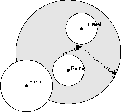
Figure 6.12:
Iterations in the locational domain. Line searches and
iterations in the stack decision variables are not depicted.
As it can be seen, the code seems to encounter some convergence problems close to the local minimum found. This might be attributed to the inevitable noise in the objective function, an effect which might also be seen in an iteration vs. function value plot, see Figure 6.13.
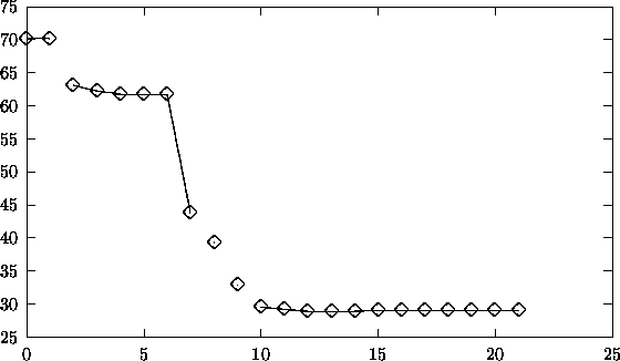
Figure 6.13: Iteration versus function values.
A notable decrease in step sizes during the iterations has not been observed,
see Figure 6.14, p. ![]() .
.
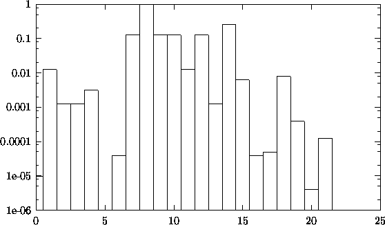
Figure 6.14: Step sizes
chosen by the optimization routine. Note that the descent direction in
iteration no. 5 was rejected.
Figure 6.15 (p. ![]() ) shows the effect
function
) shows the effect
function ![]() for the final point
for the final point ![]() overlayed over a map of the region, while Figure 6.16
(p.
overlayed over a map of the region, while Figure 6.16
(p. ![]() ) shows some approximated level curves of the
same function.
) shows some approximated level curves of the
same function.
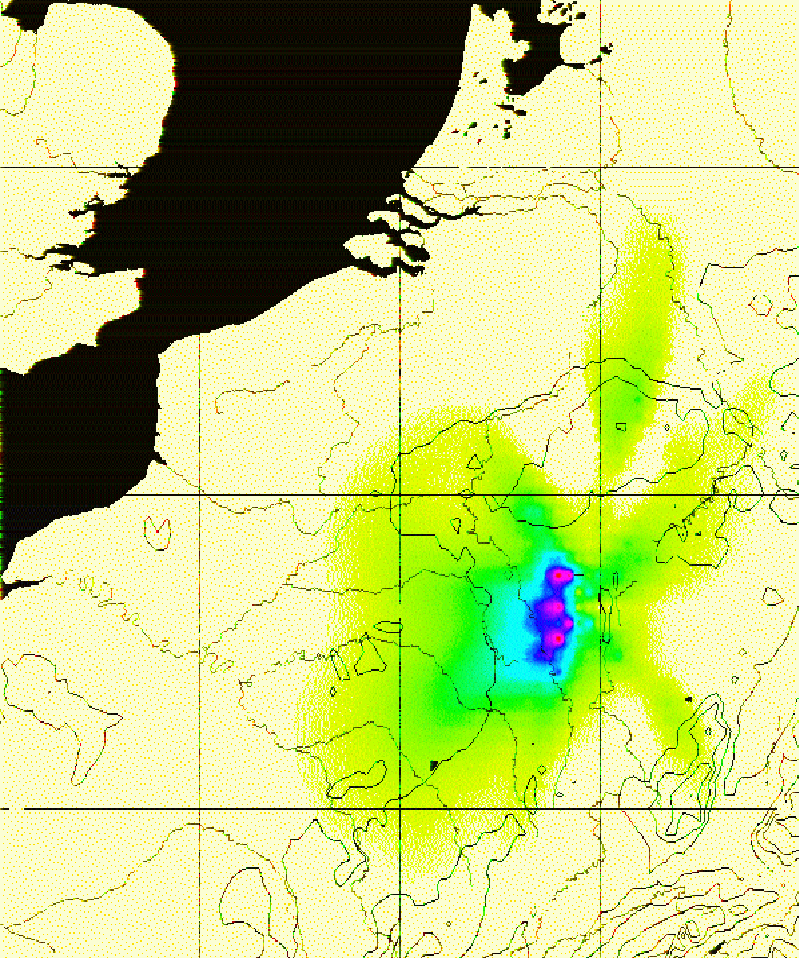
Figure 6.15: The effect function ![]() for the final
configuration.
for the final
configuration.
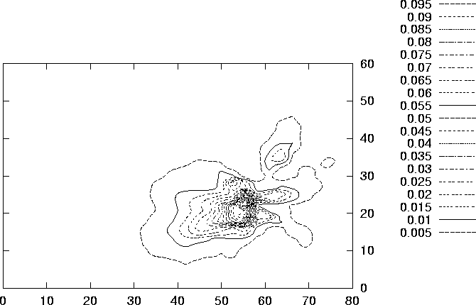
Figure 6.16: Some approximated level curves of the effect function
![]() for the final configuration.
for the final configuration.
Figure 6.17 (p. ![]() ) shows the mass of the
pollutant in different compartments at grid point (25, 19), which is a
close approximation to Paris. Similarly, Figure 6.18
(p.
) shows the mass of the
pollutant in different compartments at grid point (25, 19), which is a
close approximation to Paris. Similarly, Figure 6.18
(p. ![]() ) shows the corresponding values for the grid point
(40, 23), which is a close approximation to Reims. Moreover, the
corresponding values are plotted for
Metz (grid point (61, 21), Figure 6.19, p.
) shows the corresponding values for the grid point
(40, 23), which is a close approximation to Reims. Moreover, the
corresponding values are plotted for
Metz (grid point (61, 21), Figure 6.19, p. ![]() ),
Düsseldorf (grid point (68, 43), Figure 6.20,
p.
),
Düsseldorf (grid point (68, 43), Figure 6.20,
p. ![]() ),
and Brussel (grid point (45, 39), Figure 6.21,
p.
),
and Brussel (grid point (45, 39), Figure 6.21,
p. ![]() ).
Note that for all these figures the scales of the y-axes are differing
from picture to picture.
).
Note that for all these figures the scales of the y-axes are differing
from picture to picture.
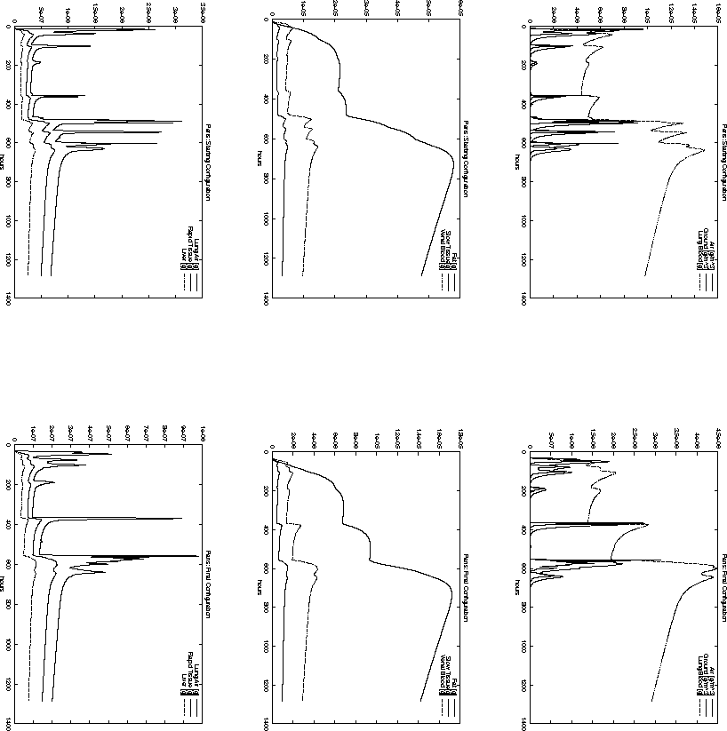
Figure 6.17: Time-dependent pollutant mass in different compartments
at Paris for the starting configuration ![]() and the final
configuration
and the final
configuration ![]() .
.
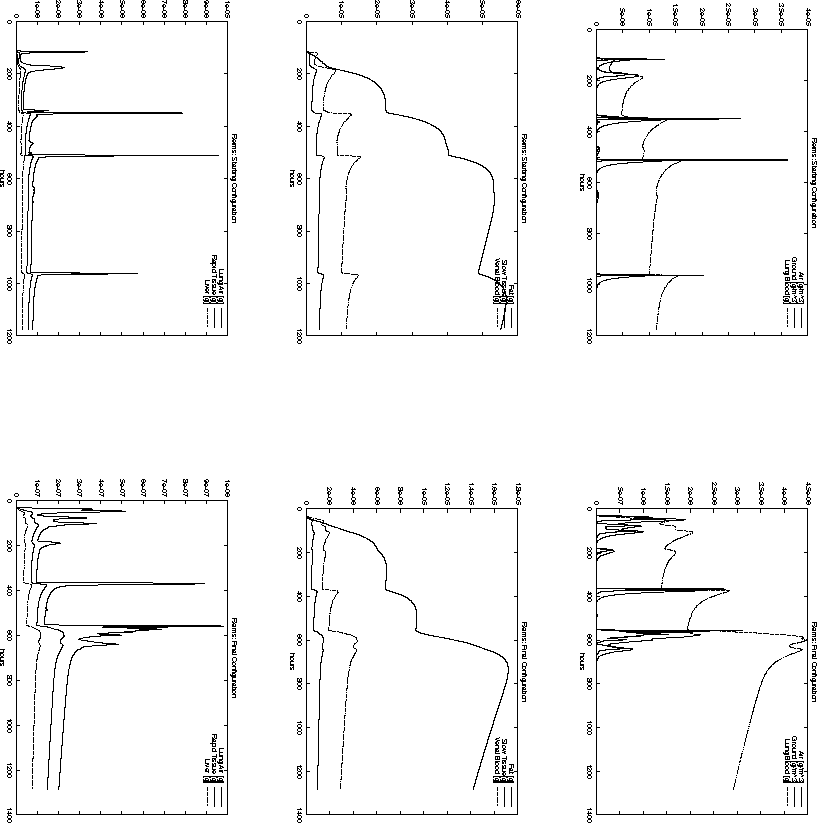
Figure 6.18: Time-dependent pollutant mass in different compartments
at Reims for the starting configuration ![]() and the final
configuration
and the final
configuration ![]() .
.
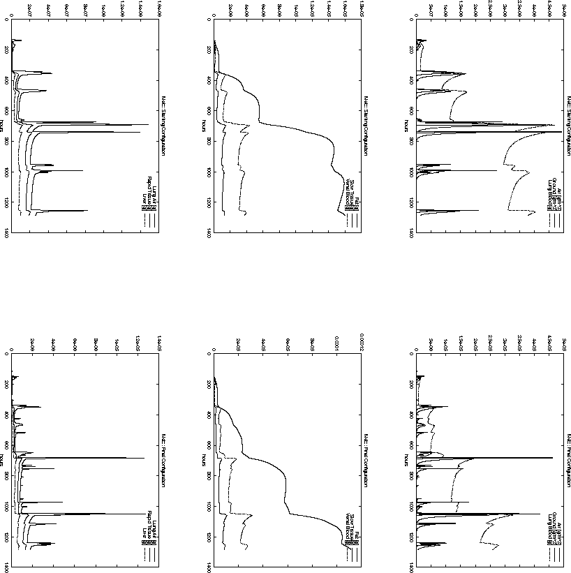
Figure 6.19: Time-dependent pollutant mass in different compartments
at Metz for the starting configuration ![]() and the final
configuration
and the final
configuration ![]() .
.
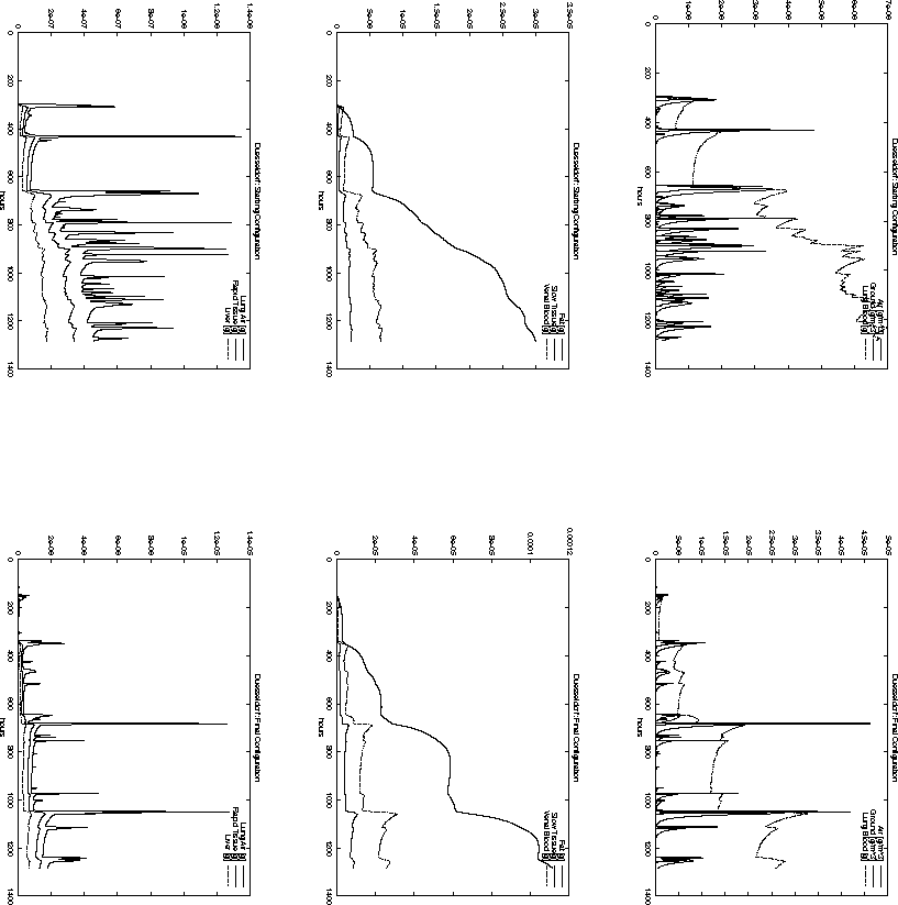
Figure: Time-dependent pollutant mass in different compartments
at Düsseldorf for the starting configuration ![]() and the final
configuration
and the final
configuration ![]() .
.
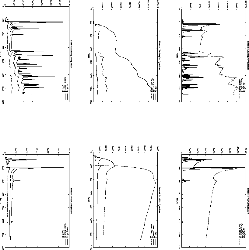
Figure 6.21: Time-dependent pollutant mass in different compartments
at Brussel for the starting configuration ![]() and the final
configuration
and the final
configuration ![]() .
.
For example, the total pollution load in Paris, Reims and Brussel is decreasing
when the starting configuration ![]() is compared to the final
configuration
is compared to the final
configuration ![]() . However, the opposite is true for the cities
of Metz and Düsseldorf. Nevertheless, the decision represented
by
. However, the opposite is true for the cities
of Metz and Düsseldorf. Nevertheless, the decision represented
by ![]() has a smaller objective function value
than
has a smaller objective function value
than ![]() . This is probably due to the high population density around
Paris. The same effect can be observed when comparing Figure 6.11
and 6.10 with Figure 6.15 and 6.16.
. This is probably due to the high population density around
Paris. The same effect can be observed when comparing Figure 6.11
and 6.10 with Figure 6.15 and 6.16.
Finally, Table 6.5 shows the profile of OLAF when run on the
data used in the case study after two function evaluations, as reported
by gprof Version 2.9.1. The work load in the optimization module
involves mainly linear algebra on matrices of dimension ![]() , so
the time spent in the corresponding routines can be neglected.
, so
the time spent in the corresponding routines can be neglected.
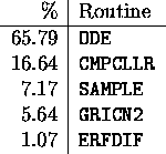
Table 6.5: Percentages
of total running time spent in subroutines. All other subroutines need less
time.
As it can be seen, most of the computation time is spent in subroutine ODE, in which the system (3.3) is solved for all grid points. Subroutine CMPCLLR, which is called from within ODE, computes the cell death and differentiation rates of the cytodynamic model described in Section 6.8. All other routines listed are subroutines of the MESOPUFF code. The table shows the typical sharp profile of a numerical analysis code, where most of the time is spent in a small number of routines, leaving ample space for further optimization and fine tuning.