Additional Notes: dstl
Statistics Workshop 23rd November 2009
Here are some additional examples raised by suggestions from workshop participants:
1. One way analysis of
variance, 1-way ANOVA
The problem below is a standard one, but a watchpoint is the way
parameters should be included in the model to avoid the problem of non-estimable
parameters.
|
DAY 0 |
DAY 1 |
DAY 3 |
DAY 5 |
DAY 7 |
DAY 14 |
DAY 21 |
|
20.1 |
20.1 |
16.6 |
15.3 |
15.8 |
17.9 |
19.6 |
|
20.5 |
16.5 |
15.8 |
17.1 |
16.5 |
17.2 |
19.1 |
|
18 |
20.1 |
16.3 |
15.8 |
16.2 |
19.4 |
18.2 |
|
19.1 |
16.9 |
18.4 |
15.1 |
18.4 |
18.1 |
19.7 |
|
17.4 |
17.5 |
16.2 |
15.4 |
16.7 |
18.4 |
18.8 |
|
17.4 |
15.8 |
16.2 |
15.5 |
17.9 |
19.2 |
19.9 |
|
18.3 |
17.7 |
16.6 |
16.3 |
14.5 |
16.7 |
|
|
17.1 |
16.2 |
16.1 |
16.3 |
16.8 |
17.1 |
|
|
19.9 |
17.5 |
17.8 |
16.4 |
18.5 |
17.3 |
|
|
19.3 |
17.6 |
16.5 |
17.5 |
18.3 |
18 |
|
|
18.7 |
16.8 |
15.8 |
18.9 |
16.2 |
16.2 |
|
|
18.2 |
17.5 |
16.5 |
16.1 |
17.4 |
19.7 |
|
|
18.6 |
18.1 |
17 |
15.7 |
17.3 |
|
|
|
18.6 |
17.2 |
16.9 |
15.9 |
15.4 |
|
|
|
18.5 |
17.3 |
16.9 |
17.2 |
15.5 |
|
|
|
18.4 |
16.8 |
18.4 |
18.7 |
15.8 |
|
|
|
19.6 |
16.1 |
17.2 |
17 |
14.3 |
|
|
|
18.1 |
16.7 |
19.3 |
18.2 |
19.5 |
|
|
|
19.3 |
18.6 |
18.3 |
15.7 |
|
|
|
|
18.6 |
18.5 |
18.8 |
14.5 |
|
|
|
|
19 |
17.3 |
18.2 |
16 |
|
|
|
|
18.9 |
17.4 |
16.8 |
18 |
|
|
|
|
20 |
16.7 |
18.6 |
16.1 |
|
|
|
|
19.7 |
16.6 |
16.5 |
19.3 |
|
|
|
|
17.9 |
19.2 |
19.2 |
|
|
|
|
|
19.9 |
16.2 |
15.8 |
|
|
|
|
|
20.5 |
18.5 |
17.1 |
|
|
|
|
|
21 |
18.1 |
18.6 |
|
|
|
|
|
18.7 |
18.7 |
17.2 |
|
|
|
|
|
18.2 |
17.4 |
17.1 |
|
|
|
|
|
18.7 |
17.4 |
|
|
|
|
|
|
19.6 |
18.2 |
|
|
|
|
|
|
19.1 |
18.6 |
|
|
|
|
|
|
18.5 |
18.5 |
|
Different n at each time point. Is
there a change in mass over time? (1-way ANOVA) |
|||
|
18.7 |
17.1 |
|
||||
|
19.6 |
18 |
|
||||
|
18.7 |
|
|
|
|
|
|
|
18.5 |
|
|
|
|
|
|
|
20 |
|
|
|
|
|
|
|
19 |
|
|
|
|
|
|
|
19.5 |
|
|
|
|
|
|
|
17.8 |
|
|
|
|
|
|
The Excel worksheet ANOVA is a simple way of checking if a
parameterization is unsatisfactory.
2. Decay Rate Example
This concerns the estimation and comparison of decay rates.
|
|
Method 1 |
|
Method 2 |
|
||
|
Time
(mins) |
Virus
1 |
Virus
2 |
Virus
3 |
|
Virus
1 |
|
|
0 |
491.4333 |
30900 |
82.26667 |
|
74 |
|
|
5 |
615.0467 |
9289.583 |
68.565 |
|
37 |
|
|
15 |
295.81 |
5175.315 |
55.33667 |
|
37 |
|
|
30 |
247.4067 |
4416.913 |
19.45 |
|
7.9 |
|
|
45 |
44.26 |
2426.28 |
12.13 |
|
7.9 |
|
|
60 |
16.06667 |
1113.45 |
9.416667 |
|
7.9 |
|
|
90 |
11.27667 |
441.5133 |
9.073333 |
|
7.9 |
|
|
|
|
|
|
|
|
|
|
|
|
|
|
|
|
|
|
|
Is there a difference between
virus decay rates? Is there a difference in methods? (regression analysis?) |
|||||
|
|
||||||
This can be modelled as a non-linear regression problem.
Alternatively by assuming multiplicative errors we can log the data and
use the linear model.
3. Poisson Regression Example
A weapon firing at a target at distance x, hits with a certain probability generating N(x) fragments.
Possible model is that
N(x)
~ Poisson(λ(x))
i.e.
Suppose
λ(x) = η(x | θ)
=  , say,
a decreasing function of x. We have data
n(x1),
n(x2),
n(x3),
....n(xm)
The loglikelihood is![]()

and θ is estimated by
maximizing the loglikelihood.
Probability weapon does not hit is
![]()
4. Combining Uncertainty
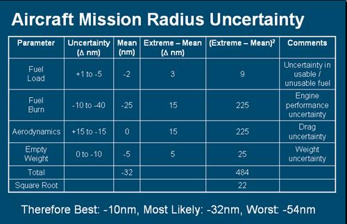
The evaluation above supposes
the sources of uncertainty are additive, giving an overall uncertainty of
Y = X1
+ X2 + X3 + X4
where the Xi are independent random
variables contributing to the total uncertainty Y.
Then the “Most Likely” variability
is based on
E(Y) = E(X1 + X2 + X3
+ X4)
= E(X1) + E(X2) + E(X3) + E(X4)
And the “Worst Case” is based
on
V(Y) = V(X1
+ X2 + X3 + X4)
= V(X1) + V(X2) + V(X3) + V(X4)
so that
SD(Y) =
SD[V(X1) + V(X2) + V(X3) + V(X4)]
A sampling approach is to
create the CDF of Y numerically by simulation.
CombiningUncertaintiesbySimulation
5. Combining information from two sensors.
How to ‘fuse’ radar and
infra-red sensor information?
Step 1: Treat each signal as
a regression:
![]()
where
εij ~ N(0, σ i2)
and the fi are probability density functions (pdf) to be fitted.
This gives estimated parameter values ![]() .
.
Step 2: Then the best (in the
sense of minimum variance) combined signal is the pdf of the random variable
where Z1 has pdf ![]() and Z2 has pdf
and Z2 has pdf ![]() .
.
If Y=aZ then f(y)dy=g(z)dz=g(z)dy/a
i.e. f(y) = g(z)/a
= g(y/a)/a.
Thus Z has pdf that is the convolution:
![]() .
.
This can be calculated numerically, or more easily by resampling.
6. Sequential Estimation of
Confidence Intervals
A common problem is the construction of a confidence interval of given
width and level of confidence. This can be tackled using a two-stage
method or a fully sequential method.
Suppose we have observations:
X1, X2,
......., Xn, .....
where each is is of the form
X = μ
+ ε, ε
~N(0, σ2)
and we wish to estimate μ
and find a confidence interval for it.
Then
![]()
and
![]() (1)
(1)
where
 and
and  . (2)
. (2)
and ![]() and
and ![]() is the upper
is the upper ![]() quantile of Student’s t distribution with
quantile of Student’s t distribution with ![]() degrees of freedom.
degrees of freedom.
The width depends on s2,
the estimate of σ 2, which is not known at the
outset.
A well-known solution is to use a two-stage method first proposed by
Stein (1945), where in the first stage one carries out a pilot set of n observations to calculate an estimate
of σ 2. Then for any
given interval width w and confidence
level α, this allows a value N to be obtained , so that if a full set
of N observations are obtained (i.e. N – n additional observations are
obtained) then a confidence interval of the desired width can be found. Stein
showed that setting the offset ![]() in (1) equal to
the desired half width can be used to find the additional number of
observations needed.
in (1) equal to
the desired half width can be used to find the additional number of
observations needed.
Stage 1: Sample n values of X, and calculate ths sample variance s2 from (1) above. Let h be the half width required (so that w = 2h).
Then set
![]()
(where ![]() denotes smallest
integer greater than or equal to z).
denotes smallest
integer greater than or equal to z).
Stage 2: Sample ![]() additional
observations, then a
additional
observations, then a ![]() % confidence interval is given by
% confidence interval is given by
 .
.
Stein’s method is not fully efficient. A better, fully sequential, way
allows observations to be added one at a time.This uses the same kind of
probability statement
![]()
as starting point where ![]() . We transform the Xi
to a sequence of independent variates (actually
. We transform the Xi
to a sequence of independent variates (actually ![]() variates when
variates when ![]() ~
~![]() ):
):
 ,
,
so that if additional observations Xn+1,
Xn+2, ... are
included then the corresponding Un,
Un+1, ...can be
added to the left hand sum in the stopping rule below without changing the
previous Ui. The stopping
rule is based on one suggested by Anscombe (1953):
Take N as the first n ( ≥
3 ) for which
 .
.
The ![]() % confidence interval is
% confidence interval is
![]()
where ![]() and
and![]() ,
,  ;
;
h1, h2 are both positive under
the condition ![]() .
.