NATCOR Simulation

Topic: Experimental Design and Analysis

Part I

1.  Introduction

The topic of experimental design and analysis is a general one, though in this course, it is being presented in the context of simulation studies. As will become plain in the next section, when we discuss metamodels, the core of the topic is statistical methodology as it applies, not simply just ot simulation models, but to all mathematical modelling where systems are being studied that are subject to random perturbations. You should therefore find the topic of much more general use than simply in simulation modelling studies, and I encourage you to adopt the approach that I will be using not only in simulation modelling but in the study of any system where random behaviour has to be accounted for.

The material that we shall study covers what I have found most useful in tackling such a modelling problem - the sort of things that in retrospect I wished had been pointed out to me when I first encountered problems of this sort.

If you have covered intermediate Statistics or OR, you may already have encountered most of the methods to be discussed. However these will usually have been taught somewhat in isolation, each within a formal, even disembodied, setting in which there is not enough scope, or time, to emphasize the overall way that these methods invariably come together when studying a simulation or a modelling problem. There is a natural way in which the methods are used, giving them a power and unity that is not always apparent when they are first encountered.

I shall try and emphasise what should be going through the mind of the investigator at each stage, showing that an overall problem can be broken down into a standard set of subproblems all of which will invariably occur, and in consequence showing that they can be tackled in a unified way.

By the end of this part of the course the student should be much more assured in the way that she/he confronts and tackles such a modelling exercise. There will be a much better awareness of the steps needed to carry out an exercise successfully, and of the problems and issues that occur at each step.

A very good book that has a similar philosophy to this course is An Introduction to Statistical Modelling by W.J. Krzanowski, (1998) Arnold, London. However this reference has a stronger statistical emphasis than we adopt and gives rather less attention to the resampling methods that we shall be using in the analysis.

Resampling is quite well covered in the book Computer Intensive Statistical Methods by J.S.U. Hjorth (1994) Chapman & Hall, London. One problem with this reference is the order in which material is presented. The initial chapters deal with arguably somewhat advanced topics. A good starting point for the book is Chapter 5.

2.  Statistical MetaModels.

This course emphasizes the importance of statistical metamodels for analysing data. We need therefore to be clear what is meant by a metamodel and this is discussed first.

Figure 2.1 illustrates the situation where we have data, Y (here and throughout this text, a quantity is written in bold to indicate that it is a vector quantity), available concerning the behaviour.of a system under study. The system itself, represented by the box in the middle, might be simple but it will typically be complicated or even unknown. We call Y the output and this is what we wish to analyse, to learn about the behaviour of the system.

We also have input quantities, whose values are expected to influence the output. The inputs are divided into two types. The input X = (X₁, X₂, … , X_k) is a vector of k explanatory variables. These are known quantities and indeed may possibly be under the control of the investigator. The input θ = (θ₁, θ₂, …, θ_p) is a vector of parameters which influence the output but whose values are not controllable. Often they will be unknown. Their values would therefore have to be estimated.

In addition the output Y may contain a random component, typically referred to as ‘noise’ or ‘error’. This is denoted by ε.

Figure 2.1: Schematic of the System

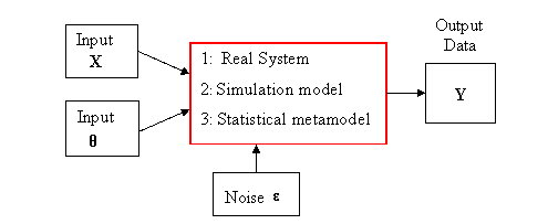
As well as depicting the situation where the output data has been obtained from a real system Figure 2.1 also illustrates the situation where we have constructed a simulation model and have made simulation runs with it to obtain simulated output data. This is indicated in Figure 2.1 by replacing the real system in the central block by a simulation model. All other blocks remain the same.

In this course the focus is on how to analyse Y and in particular to identify how the inputs X and  influence Y in the presence of the random effects . We use a statistical model for doing this. We shall make precise later what is meant by a statistical model. However we observe here that the structure of the process is unchanged, and this is emphasized by using Figure 2.1 yet again, only with the central block now representing the statistical model.

The term statistical model is conventionally used when we are analysing data obtained from a real system. In the case of data obtained from a simulation model, then the statistical model is a model of a model, so to speak – and this is when the term metamodel is used. It will be clear that whatever statistical model is deemed appropriate in a given situation is determined purely by the structure of the data and not by its origin. Thus the model would apply whether the output came from a real system or a simulation model.

Example 2.1: Consider the operation of a queue where we are interested in estimating, the average queue length, over a given period of time, T say. Here Y might be the sampled mean queue length over a period of length T. Input quantities are λ the arrival rate, and μ, the service rate, and C might be the number of servers available.  Traffic Queue Length EG

This is a situation that has been well analysed theoretically and where the relationship between Y and the quantities λ, μ and C is known precisely in certain situations. However we might be uncertain about the precise form of inter-arrival and service time distributions. We can assume that the results of n simulation runs take the form

                                                 (2.1)

where  is some suitably selected function characterising the likely behaviour of Y. The quantity  is a random variable. A common assumption is that the errors have a normal distribution:

~ .                                                                                  (2.2)

This assumption is questionable in the present context as the variability of Y will depend critically on the traffic intensity , so the assumption of constant variance  for the observations Y  is dubious.                                                              □

Example 2.2: The National Health Service has data for, Y, the number of newly registered diabetics in each year for a given number of years. It also has data on a selection of factors that might influence the onset of diabetes such as, X₁ amount of alcohol consumed; X₂ the number of cigarettes smoked, per day; X₃; previous illnesses contracted, age, sex of each case. The problem here is to those identify factors that have a significant influence on the onset of diabetes. A typical model is

.                   (2.3)

where y_i is the observed number of registered diabetics in year i  and x_ij is the observed value of the jth factor in year i; and we have n years of observations. Again we might assume normal errors  ~ .                                                           □

The scenario of Figure 2.1 can be varied or extended in many different ways. We illustrate this with two commonly occurring situations.

The first is illustrated in Figure 2.2. This is the situation where the input θ parameters can be estimated using data or past information, w, containing information about θ. Sometimes this information is not explicit but is derived from expert opinion. The estimation in this latter case is then possibly subjective. We write these estimates as , or simply as  depending on whether past data w is involved or not, using the circumflex to indicate an estimated quantity.

Figure 2.2: Input Parameters Estimated from Data

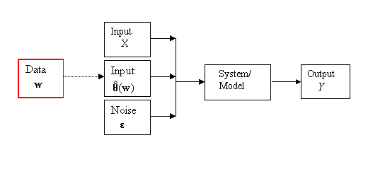
Example 2.1 (continued): It may be that λ, the arrival rate, is not known. However we have a sample of interarrival times from which λ can be estimated.                    □

Another important variation is when a dynamic system or simulation is being examined. Here time - which we denote by t - enters into the picture. It is usually best to treat t as being a continuously varying input variable that is part of the input X, but which then results in the output Y being time-dependent. Figure 2.3 represents this time dependent situation.

Figure 2.3: Schematic of a Dynamic System/Model

Data

w

   System/

   Model

Output

Noise

ε

Input

Input

    X

Example 2.3: In the study of an epidemic let η(t, θ) represent the prevalence of a certain disease at time t. (Prevalence means the proportion of the population who has the given disease.) Several scenarios are possible. Firstly, it may be that there is no information on θ, but there are observations y_i of the prevalence at given time points t_i i =1, 2, ..., n. These are subject to error, thus

y_i = η(t_i, θ) + ε_i,         i =1, 2, ..., n.                                             (2.4)

Then the problem would be to fit θ to the observations {y_i}. Secondly we might have past information w on which θ depends and the task is then to estimate θ from the information w. The third possibility is when we have both observations {y_i} of the epidemic and there is past information w on the parameters θ. In this case we should use both the {y_i} and w to estimate θ.

The following is a set of data giving the number of notifications of pulmonary TB (per 100,000) in Morocco in four selected years 1980, 1986, 1993, 2000, grouped by age.  What form should η(t, θ) take? Moroccan TB Data                                          □

In dynamic problems the regression formulation (4) is typical. The regression function η(t, θ) has to be selected so that its behaviour resembles the output of the system or mathematical/simulation model that it represents. In some situations, as might occur in the dynamic case just considered, the physical process of the actual system may be sufficiently known to suggest a natural form for η(t, θ).

Example 2.4: The logistical curve

                                                                 (2.5)

is commonly used to represent population growth when this takes a sigmoidal form. □

Exercise 2.1: Plot the logistic curve on a spreadsheet for different combinations of α, β, γ.                                                                                                                              □

If little is known about the real system, the form assumed for η(t, θ) does not have to be complicated. When there is a single explanatory variable X then a low polynomial function of X is a typically used model:

                                                         (2.6)

When there are a large number of factors, and especially when the errors ε are not small then a multivariate linear form is often used:

                                                    (2.3 bis)

Here the x_i are the values of the different factors, and the model only considers the inclusion of a linear term for each factor.  Example 2.2 is an illustration of a situation where this multivariate form is appropriate.

Sometimes the output Y takes a binary form, indicating success (Y = 1) or failure (Y = 0). Representing Y in terms of a continuous function is not then very sensible. The usual ploy is to model the probability π that Y = 1 and then to ensure that π lies between 0 and 1 by using a transformation such as the logistic transformation. This is usually written as

                                         (2.7)

but the more correct version is

                                      (2.8)

as (in the one x variable case) it is actually

                                                                (2.9)

that is the logistic transform.

This binary model is best not thought of in regression terms. Instead we regard each observation as a Bernoulli variable

Y_i ~ Bernoulli( )                                                              (2.10)

Example 2.5: An example of binary response data: Vaso Constriction Data

As far as this course is concerned we will be focusing on the third representation of Figure 2.1 where we use a statistical model to describe the output. The first step in model formulation is therefore to write down the distributional form of the output and in particular to make explicit how the distribution is expected to depend on the input quantities. It should be stressed that the statistical model does not have to precisely copy the characteristics of the underlying true model, which anyway may be too complicated to be sensibly reproducible. Rather the statistical model has to be capable of modelling the essential features of the system it represents, but that is all that is needed. Figure 2.4 illustrates this key requirement, in the dynamic case, by including boxes to represent both the unknown system and the statistical model representing it. The parameters  of the statistical model do not have to correspond in any explicit way to the parameters θ of the system, and this is indicated in Figure 2.4

Often the regression format is a convenient one to use. However, as the last example shows, the regression approach is not completely general. In fact the procedure used in equation (2.8) of the last example, of treating Y as a random variable and writing down its distribution by name, is a very good one to follow. The distribution will usually depend on parameters. It is also necessary therefore to write down how these parameters of the distribution depend on the input variables and on the input parameters of the process model.

Figure 2.4: This depicts a Statistical Model of a System.

It also depicts a Metamodel of a Simulation Model

Statistical Model..

Output

Output

Input

    X

System/

   Model

Input

Data

w

Noise

U

The main conclusion to draw from our consideration of statistical metamodels is summarized in the following :

The first step of treating the output Y as a random variable, and of identifying its distribution, is essential in determining the most appropriate subsequent analysis.

We discuss the main characteristics of random variables in Part II.