Computer
Analysis of Models
1. Introduction
This course aims to bring together modelling and statistical methodology in the way that it is actually used in practice. The course provides the student with the information and viewpoint that I have found most useful in tackling a modelling problem - the sort of things I wished had been pointed out to me when I first started tackling poblems of this sort.
Those near the end of an MSc programme in either Statistics or OR will already have encountered most of the methods used in this course. However these will usually have been taught somewhat in isolation, each within a formal, even disembodied, setting in which there is not enough scope, or time, to emphasise the overall way that these methods invariably come together when studying a modelling problem. There is a natural order in which the methods are used, giving them a power and unity that is not well appreciated by students. Indeed it is often totally lost on them.
This course aims to revisit statistical and modelling methodology in a way that emphasises how they are used in practice. It emphasises what should be going through the mind of the investigator at each stage. The overall problem can be broken down into a standard set of subproblems all of which will invariably occur. Each subproblem will be reviewed and discussed, not in an isolated way, but in the context of the overall problem.
By the end of the course the student should be much more assured in the way that she/he confronts and tackles such a modelling exercise. There will be a much better awareness of the steps needed to carry out an exercise successfully, and of the problems and issues that occur at each step.
A very good book
that has a similar philosophy to this course is An Introduction to Statistical
Modelling by W.J. Krzanowski (1998)
2. Random Variables
The key concept of all statistics is the random variable. A formal definition of
a random variable requires a mathematical foundation (and elaboration) that
takes us away from the main focus of this course. We shall therefore not
attempt a formal definition but instead adopt a simpler practical viewpoint. We
therefore define a random variable simply as a quantity that one can observe many
times but that takes different values each time it is observed in an
unpredictable, random way. These values however will follow a probability distribution. The
probability distribution is thus the defining property of a random variable.
Thus, given a random variable, the immediate and only question one can, and
should always ask is: What is its distribution?
We denote a random variable by an upper case
letter X (Y, Z etc.). An observed value of such a random variable
will be denoted by a lower case letter x
(y, z etc).
In view of the above discussion, given a
random variable, one should immediately think of the range of possible values that it can take and its probability distribution over this range.
The definition of most statistical
probability distributions involves parameters.
Such a probability distribution is completely fixed once the parameter values
are known. Well known parametric probability distributions are the normal,
exponential, gamma, binomial and Poisson.
A probability distribution is usually either discrete or continuous. A discrete distribution takes a specific set of values,
typically the integers 0, 1, 2,…. Each value i has a given probability pi
of occurring. This set of probabilities is called its probability mass function.
Exercise: Plot the probability mass
function of
(i)
the binomial distribution, B(n,
p)
(ii)
the Poisson distribution, P(λ)
Write down what you know of each
distribution.
A continuous random variable, as its name
implies, takes a continuous range of values for example all y ≥ 0. One way of defining its distribution
is to give its probability density
function (pdf), typically written as f(y). The pdf is not a probability, however it can be used to form a probability increment. ![]() This is a good way to
view the pdf.
This is a good way to
view the pdf.
Exercise: Write down the pdf of
(i) the
normal distribution, ![]() . Answer:
. Answer: ![]()
(ii) the gamma distribution, ![]() . Answer:
. Answer: ![]()
Plot the density functions. Write down what
you know about each distribution.
Exercise: Suppose that X is a continuous random variable with density f(x). Let Y be a function of X, say Y = h(X).
What is the pdf, g(y) of Y, in terms of f(x)? Give the pdf of Y = X 2 when X is a standard normal random variable.
What is the name of this random variable and what is the form of its pdf?
An alternative way of defining a probability
distribution, which applies to either a discrete or continuous distribution, is
to give its cumulative distribution
function (cdf).
Exercise: Write down the main properties
of a cdf.
Exercise: Plot the cdf’s of each of the
examples in the previous examples.
Exercise: What is the relation between the
pdf and the cdf for a continuous random variable? How is one obtained from the
other?
Exercise: Define the expected value of a random variable X in terms of its pdf f(x). Define the expected value of Y = h(X) in terms of the pdf of X.
3. Fitting
Parametric Distributions to Random Samples
Random samples are the simplest data sets that are encountered. A random sample is just a set of n independent and identically distributed observations (of a random variable). We write it as Y = {Y1, Y2, … Yn,} where each Yi represents one of the observations.
Exercise: Generate random samples from
(i)
the normal distribution ![]() .
.
(ii)
the gamma distribution ![]() . GammaVarGenerator
. GammaVarGenerator
A basic problem is when we wish to fit a parametric distribution to a random sample. This problem is an elementary form of modelling called input modelling.
Example: Suppose we are modelling a queueing system where service times are expected to have a gamma distribution and we have some actual data of the service times of a number of customers from which estimate the parameters of the distribution. This is an example of the input modelling problem. If we can estimate the parameters of the distribution, we will have identified the distribution completely and can then use it to study the characteristics of the system employing either queueing theory or simulation.
To fit a distribution, a method of estimating the parameters is needed. The best method by far is the method of maximum likelihood (ML). The resulting estimates of parameters, which as we shall see shortly possess a number of very desirable properties, are called maximum likelihood estimates (MLEs). ML estimation is a completely general method that applies not only to input modelling problems but to all parametric estimation problems. We describe the method next.
4. Maximum
Likelihood Estimation
Suppose Y = {Y1, Y2,
…, Yn} is a set of
observations where the ith
observation, Yi, is a
random variable drawn from the continuous distribution with pdf fi(y, θ) (i = 1,2, …, n). The subscript i
indicates that the distributions of the yi
can all be different.
Example: Suppose Yi ~ N(μ, σ 2) all i. In this case
![]()
so that the observations are identically distributed. The set of observations is therefore a random sample in this case.
Example: Suppose Yi ~ ![]() . In this case one often writes
. In this case one often writes
![]() where
where ![]() ~ N(0, σ 2)
~ N(0, σ 2)
The pdf of Yi is
![]() .
.
This is not a random sample in this case, because the observations are not all identically distributed. However ML estimation will still work in this case.
The ML method works as follows.
Suppose that y = {y1, y2, …, yn} is a sampled value of Y = {Y1, Y2, …, Yn}. Then we write down the joint distribution of Y evaluated at the sampled value y as:
![]() .
.
This expression, treated as a function of θ, is called the called the likelihood (of the sampled value y). The logarithm:
![]()
is called the loglikelihood.
The ML estimate, ![]() , is that value of
, is that value of ![]() which maximizes the loglikelihood.
which maximizes the loglikelihood.
In some many cases the maximum can be obtained explicitly as the solution of the equation
![]()
which identifies the stationary points of the
likelihood. The maximum is often obtained at such a stationary point. This
equation is called the likelihood
equation.
In certain situations, and this includes some
well known standard situations, the liekelihood equations can be solved to give
the ML estimators explicitly. This is preferable when it can be done. However
in general the likelihood equations are not very tractable. Then a much more
practical approach is to obtain the maximum using a numerical search method.
There exist a number of powerful numerical optimizing
methods but these can be laborious to set up. An exception is the readily
accessible numerical optimizer Solver
which can be called from an Excel spreadsheet. This can handle problems that
are not too large. A more flexible alternative is to use a direct search method
like the Nelder-Mead method. This is
discussed in more detail in the Appendix.
Example: NelderMeadDemo This is a VBA
implementation of the Nelder-Mead Algorithm. Insert a function of your own to
be optimized and see if finds the optimum correctly. Watchpoint: Check whether
an optimizer minimizes or maximizes the objective. Nelder Mead usually does
function minimization.
Example: The following is a (random)
sample of 47 observed times (in seconds) for vehicles to pay the toll at a
booth when crossing the
An important property of the MLE, ![]() , is that its asymptotic probability distribution
is known to be normal
, is that its asymptotic probability distribution
is known to be normal
![]() ~
~ ![]()
where ![]() is the unknown true parameter value and the variance has the form
is the unknown true parameter value and the variance has the form
 .
.
This is not known, as it depends on ![]() which is the unknown, but it can be approximated by
which is the unknown, but it can be approximated by
 .
.
The expectation is with respect to the joint distribution of Y and can be hard to evaluate. In practice the approximation
![]() '
'![]()
is quite adequate; or at least it will give an initial indication of the variability of the MLE. Thus the working version of (???) is
![]() ~
~ ![]()
The expression ![]() can be very messy
to evaluate analytically. Again it is usually much easier to calculate this
numerically using finite-difference formulas for the second derivatives. The
expression is a matrix of course, and the variance-covariance matrix of the MLE
is the negative of its inverse. A
numerical procedure is needed for this inversion.
can be very messy
to evaluate analytically. Again it is usually much easier to calculate this
numerically using finite-difference formulas for the second derivatives. The
expression is a matrix of course, and the variance-covariance matrix of the MLE
is the negative of its inverse. A
numerical procedure is needed for this inversion.
The way that (???) is typically used is to provide confidence intervals. For example an (1-α)100% confidence interval for the coefficient θ1 is
![]()
where ![]() is the upper 100α/2 percentage point of the standard
normal distribution.
is the upper 100α/2 percentage point of the standard
normal distribution.
Often we are interested not in θ directly, but some arbitrary, but given function of θ, g(θ) say. ML estimation has the attractive general invariant property that the MLE of
g(θ) is
![]() .
.
An approximate (1-α)100% confidence interval for g(θ) is then
![]()
In this formula
the first derivative of g(θ) is required. If this is not
tractable to obtain analytically then, as with the evaluation of the
information matrix, it should be obtained numerically using a finite-difference
calculation.
Summarising it will be seen that we need to
(i) Formulate a statistical model of the data to be examined. (The data may or may not have been already connected. The data might arise from observation of a real situation, but it might just as well be collected from a simulation.)
(ii) Write down an expression for the loglikelihood of the data, identifying the parameters to be estimated.
(iii) Use this in a (Nelder-Mead say) numerical optimization of the loglikelihood..
(iv) Use the optimal parameter values to obtain estimates for the quantities of interest.
(v) Calculate confidence intervals for these quantities.
Example: Suppose that the gamma
distribution ![]() fitted to the toll
booth data of example (???) is used as the service distribution in the design
of an M/G/1 queue. The interarrival time distribution is known to be
exponential with pdf
fitted to the toll
booth data of example (???) is used as the service distribution in the design
of an M/G/1 queue. The interarrival time distribution is known to be
exponential with pdf
![]()
but a range of possible values for the
arrival rate, λ, needs to be
considered.
Plot a graph of the mean waiting time W(λ) for the queue for 0 < λ < 0.1 (per second), assuming
that the service time distribution is gamma: ![]() . Add 95% confidence intervals to this graph to take into
account for the uncertainty concerning
. Add 95% confidence intervals to this graph to take into
account for the uncertainty concerning ![]() because estimated values
because estimated values ![]() have been used.
have been used.
The previous example contains all the key steps in fitting a statistical model to data. There are several additional aspects that we
3. Empirical Distribution Functions
Consider first a
single sample of observations ![]() , for i = 1, 2,
..., m. (These might be a set
of outputs from a number of ATLAS runs, say, all made under ostensibly the same
conditions.) The EDF is defined as:
, for i = 1, 2,
..., m. (These might be a set
of outputs from a number of ATLAS runs, say, all made under ostensibly the same
conditions.) The EDF is defined as:
![]() . (1)
. (1)
The EDF is illustrated in Figure 2. It is usually simplest to think of the observations as being ordered:
Y(1) < Y(2) < … < Y(m) . (2)
Figure
2: EDF of the Yi , ![]()
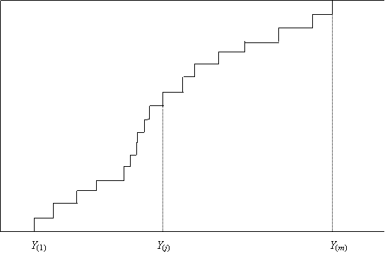
These are what are depicted in Figure 2. Note that the subscript are placed in brackets to indicate that this is an ordered sample.
The key point is that the EDF estimates the (unknown) cumulative distribution function (CDF) of Y. We shall make repeated use of the following:
Fundamental Theorem of Sampling: As the size of a random sample tends to infinity then the EDF constructed from the sample will tend, with probability one, to the underlying cumulative distribution function (CDF) of the distribution from which the sample is drawn.
(This result when stated in full mathematical rigour, is known as the Glivenko-Cantelli Lemma, and it underpins all of statistical methodology. It guarantees that study of increasingly large samples is ultimately equivalent to studying the underlying population.)
We consider how the EDF can be used for comparing the output of simulation runs using different models. As already mentioned, the attraction of using the EDF directly, rather than a fitted CDF, say, is that we make no assumption about the underlying distributional properties of Y. Thus Y can be either a continuous or a discrete random variable. Nor is it assumed to come from any particular family of distributions like the normal or Weibull. This flexibility is particularly important when studying or comparing the output from complex simulations where it is possible that the distribution of the output may be unusual. For example it may well be skew, or possibly even multimodal.
5. Bootstrap
Method
The basic
process of constructing a given test statistic is illustrated in Figure 3. This
depicts the steps of drawing a sample Y =
(Y1, Y1, ..., Ym)
of size m from a distribution F0(y), and then the calculating the statistic of interest T from Y. The problem is then to find the distribution of T.
Bootstrapping is a very general method for numerically estimating the distribution of a (test) statistic. It is a resampling method that operates by sampling from the data used to calculate the original statistic.
Bootstrapping is based on the following idea. Suppose we could repeat the basic process, as depicted in Figure 3, a large number of times, B say. This would give a large sample {T1, T2,..., TB} of test statistics, and, by the Fundamental Theorem of Section 3, the EDF of the Ti will tend to the CDF of T as B tends to infinity. Thus, not simply does the EDF estimate the CDF, it can be made accurate to arbitrary accuracy at least in principle, simply by making B sufficiently large.
Figure 3: Basic Sampling
Process

Unfortunately to apply this result requires repeating the basic process many times. In the present context this means having to repeat the simulation trials many times - something that is certainly too expensive and impractical to do.
The bootstrap method is based on the idea of replacing F0(.) by the best estimate we have for it. The best available estimate is the EDF constructed from the sample Y. Thus we mimic the basic process depicted in Figure 3 but instead of sampling from F0(.) we sample from the EDF of Y. This is exactly the same as sampling with replacement from Y. We carry out this process B times to get B bootstrap samples Y*(1), Y*(2), ..., Y*(B). (We have adopted the standard convention of adding an asterisk to indicate that a sample is a bootstrap sample.) From each of these bootstrap samples we calculate a corresponding bootstrap test statistic value T*(i) = T(Y*(i)), i = 1, 2, ..., B. The process is depicted in Figure 4.
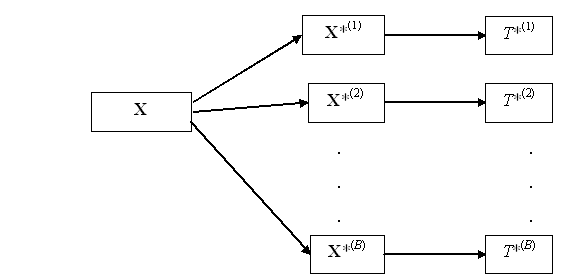
Figure 4: Bootstrap Process
The EDF of the bootstrap sample, which without loss of generality we can assume to be reordered, so that T*(1) < T*(2) < ... < T*(B), now estimates the distribution of T. This is depicted in Figure 5. Figure 5 also includes the original test statistic value, T0. Its p-value, as estimated from the EDF, can be read off as
![]() . (11)
. (11)
If the p-value is small then this is an indication that the two samples are not drawn from the same distribution.
In practice
typical values of B used for
bootstrapping are 500 or 1000, and such a value is generally large enough. With
current computing power resampling 1000 values (which is the default value used
in the our spreadsheet demonstrations) is, to all intents and purposes,
instantaneous. A good reference for bootstrap methods is Davison and Hinkley
(1997).
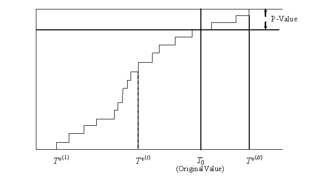
Figure 5: Empirical Distribution Function of the T(i)
Models
The final example of the previous section
captures the key features of a statistical analysis.
We will need to review the tools and
techniques at our disposal, however we follow the precepts set out in the
introduction and get to grips with a typical modelling problem immediately.
This is how it is in practice. Imagine we are a consultant with our customer
standing in front of us. She/he will not be interested in our inspecting and
reviewing the tools at our disposal. Our first step is to look at the system
that is the object of our attention. Some examples are
1. An epidemic
2. A queuing system
3. A production process
4. A supply chain
5. A project and its management
6. An environmental system
7. A battle
7. A mechanical/engineering system
The main purpose of a typical OR study might
very well be to construct a mathematical or a simulation model of such a system
in order to study its behaviour. However in this course, this is not the issue
of interest. We shall not be
discussing the construction of such a model, but will regard such a model as a
‘black-box’. Our view of the system is as given in Figure 1
Figure 1: Schematic of the System/Model
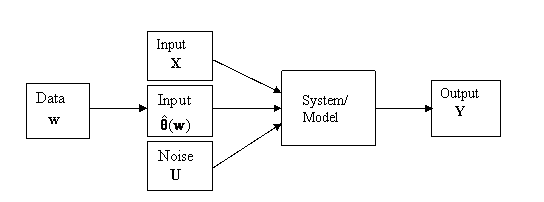
The inputs are divided into two types. The
input X = (X1, X2, … , Xk) is a vector of k
explanatory variables. These are known quantities and indeed may possibly be
selectable by the investigator. The input θ = (θ1, θ2,
…, θp) is a vector of
unknown parameters. These will therefore have to be estimated. This is done using separate data or past information, w,
containing information about θ. Alternatively the estimation might
be subjective, and be derived from expert opinion. We write these estimates as ![]() , or simply as
, or simply as ![]() depending on whether
past data w is involved or not, using the circumflex to indicate an
estimated quantity. In addition there may be a random component, typically
referred to as ‘noise’ or ‘error’ which affects sytem performance. This has
been denoted by U to indicate that in a simulation model this error is
introduced by transforming uniform random variables.
depending on whether
past data w is involved or not, using the circumflex to indicate an
estimated quantity. In addition there may be a random component, typically
referred to as ‘noise’ or ‘error’ which affects sytem performance. This has
been denoted by U to indicate that in a simulation model this error is
introduced by transforming uniform random variables.
Example:
The schematic of Figure 1 can be used to
represent the system in two distinct
ways. It can represent:
(i)
The actual system itself
or
(ii) A mathematical or simulation
model of the system
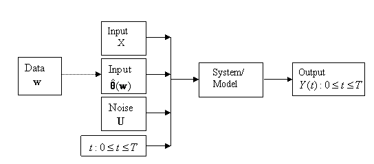
Figure 1 is a generic model only, and there
are variations. One important variation, when a dynamic system or simulation is
being examined, is the way time -
which we denote by t - enters into
the picture. It is usually best to treat t
as being a continuously varying input variable that is part of the input X,
but which then results in the output Y being time-dependent. Figure 2
represents this time dependent situation.
Figure 1 is a generic model only, and there
are many variations. One important variation, when a dynamic system or
simulation is being examined, when we introduce time, which we denote by t,
explicitly into the scheme. It is usually best to treat t as being a continuously varying input variable that is part of
the input X, but which then results in the output Y being
time-dependent. Figure 2 represents this time dependent situation.
Figure 2: Schematic of a Dynamic System/Model
There is a third way of representing the
system. This uses a statistical model.
This can represent either (i) the
actual system or (ii) the
mathematical or simulation model. In case (ii) it is then called a metamodel because it is a model of a
model!
As far as this course is concerned we will be
focusing on this third representation. We shall not slavishly call it a
metamodel, but simply call it a statistical model for short with the understanding
that it is always a metamodel.
Whether it is a statistical model of the
actual system or of a mathematical/simulation model of the system will depend
on the context. The important thing is that the statistical model will need to
contain the right structure to explain the relationship between the inputs X
and ![]() and the output Y.
But this structure needs to be developed at the metalevel and not involve
detailed causal relationships of the actual system.
and the output Y.
But this structure needs to be developed at the metalevel and not involve
detailed causal relationships of the actual system.
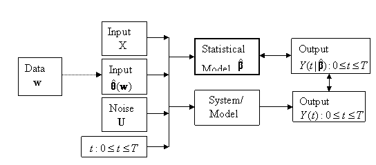
The statistical model needs to be set up so
that its output resembles the output of the system or mathematical/simulation
model that it represents. This is done by fitting
it to given input data X and ![]() and output data Y, this
latter either being real output or output obtained from a mathematical or
simulation model. The situation corresponding to Figure 2 is depicted in Figure
3. There will usually be uncertainty as the form of the statistical model. This
is handled by including some adjustable parameters or coefficients, β,
in the statistical model. Fitting the model therefore requires estimating the β. The
estimates,
and output data Y, this
latter either being real output or output obtained from a mathematical or
simulation model. The situation corresponding to Figure 2 is depicted in Figure
3. There will usually be uncertainty as the form of the statistical model. This
is handled by including some adjustable parameters or coefficients, β,
in the statistical model. Fitting the model therefore requires estimating the β. The
estimates, ![]() , are found by ensuring that the output of the statistical
model closely resembles the output of the system or model.
, are found by ensuring that the output of the statistical
model closely resembles the output of the system or model.
Figure 3: Fitting a Statistical Metamodel to
Data from a Dynamic System/Model
We shall use the regression approach to analysis of simulation output. [Use quadratic regression example, and PAD example. Mention basic estimation formulas.]
Static or Dynamic models and their dependence on structural parameters.
Input models and Selecting input distributions.
Output
Analysis
Regression Metamodels
Fitting
Models to Data (Simulated or Real)
Likelihood Methods. Numerical Optimization
Effects of
Parameter Variability, Simulation Variability
Validating
Models with Real Data
Examples of
1. Epidemic Model
2. Toll Booth Queue Model (Input Model)
3. Financial Forecast Model (TimeSeries with Regression)
4. Aircraft Scheduling Model
5. Project Management under Uncertainty